A Journey Through Statistical Mechanics (Part 1): Counting Our Way to Temperature

This is Part 1 of a two-part series. Part 1 (this one): the single axiom thermal physics rests on, and how counting microstates forces temperature, pressure, and free energy into existence. Part 2: the great reversal — partition functions, Gibbs sums, and the quantum statistics that ends with Bose–Einstein condensation and Fermi seas.

Let me start with something you have stared at a hundred times: a glass of water sitting perfectly still on a table. To the eye it is the very picture of calm. Yet underneath that calm, $10^{23}$ particles are colliding, swapping places, and flinging energy back and forth in a storm we have no hope of tracking. Classical physics, faced with this, would want to chase every trajectory. Thermal physics makes a wiser bet: stop tracking the dancers and listen to the rhythm of the whole crowd.

That is the move I want to follow in this series, because it is one of the cleanest examples of More is Different in all of physics. We are not going to memorize a zoo of formulas. We are going to plant one absurdly simple assumption and watch the entire edifice of thermodynamics — temperature, pressure, chemical potential, free energy — grow out of it on its own, like dominoes falling in sequence. (A word of warning before we set off: I will assume you have met quantum mechanics, because statistical mechanics is quantum at heart. What we are really doing, all along, is counting the statistical effects of staggering numbers of quanta.)

image 1.png

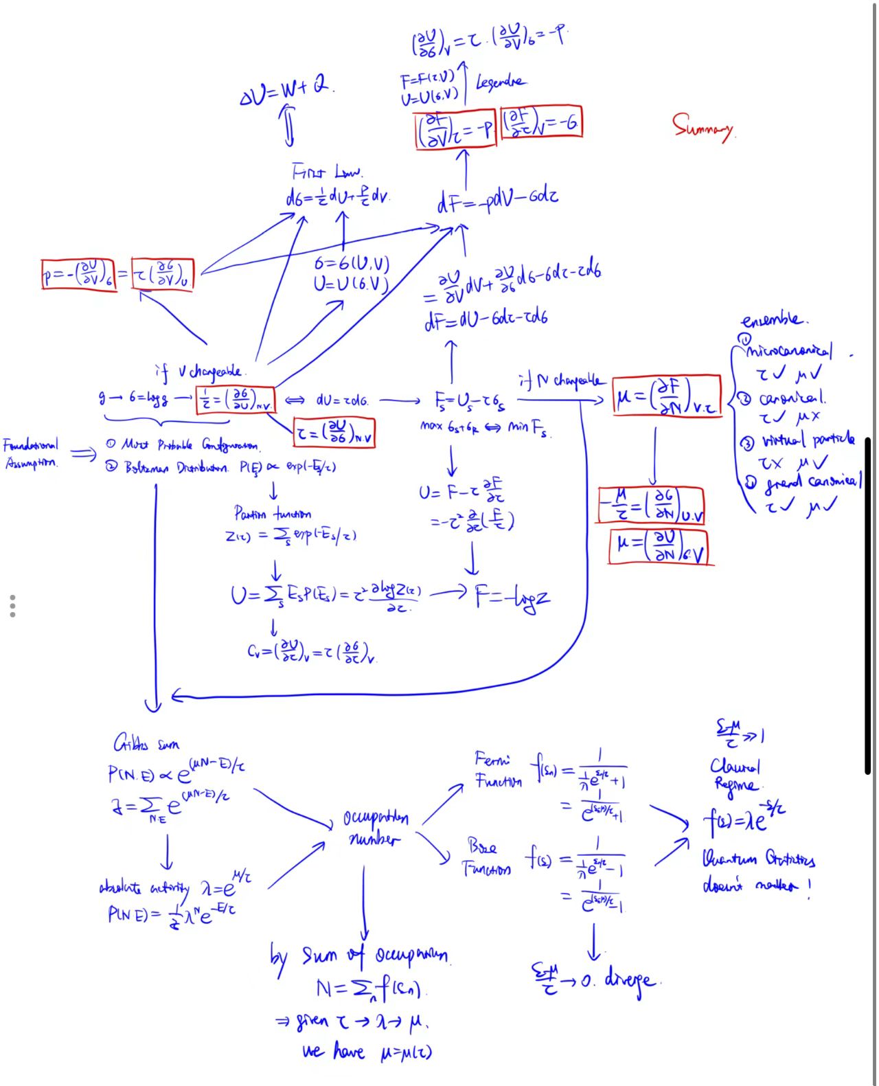
1. The Art of Counting — from multiplicity to thermal equilibrium

Our journey begins with a question so simple it sounds almost childish: under fixed macroscopic conditions, how many microscopic “ways of being” does a system actually have? Physicists give that count a name — the multiplicity, written $$g$$ .

The fundamental assumption: Nature is fair

Picture an isolated box holding $$N$$ particles, with total energy $$U$$ and volume $$V$$ . The particles are careening around, colliding without pause. One instant particle A is on the left and B is on the right; the next instant they have traded places. Out of this chaos, statistical mechanics asks us to accept exactly one axiom — the fundamental assumption:

For an isolated system, all accessible quantum states that conserve energy occur with equal probability.

That is the whole creed. Nature plays no favorites: as long as the energy budget allows it, finding the system in state A is exactly as likely as finding it in state B. Everything else in this article is bookkeeping built on top of that one sentence.

Why bother defining entropy? ( $S = \ln g$ )

Here is a fair objection. If multiplicity $$g$$ already counts the states, why invent “entropy” at all? Not for mystique — for two thoroughly practical reasons.

First, the numbers are monstrous. For anything macroscopic, $$g$$ is astronomical; even a small vial of gas can reach an order of magnitude like $10^{10^{23}}$ . You cannot do honest arithmetic with a tower like that.

Second, we want additivity. Take two glasses of water, systems A and B. Counted as one combined system, the total number of states is the product of the parts, $g_{total} = g_A \times g_B$ , because every state of A can pair with every state of B. But macroscopic physics runs on addition — mass adds, volume adds, energy adds. We would like our measure of “disorder” to add too.

What single operation turns multiplication into addition and tames a runaway exponent into something human-sized? The logarithm. So Boltzmann (and Planck) handed us one of the most quietly profound definitions in physics, the fundamental entropy:

\sigma = \ln g

That is all entropy is, at bottom: the logarithm of the number of microstates. Not a mysterious destructive force, just our yardstick for a system’s “number of possibilities.”

Why thermal equilibrium is maximum entropy

Now for the moment the machinery first earns its keep. Set two independent systems A and B side by side and let them make thermal contact — they may trade energy, but the total $U_{total} = U_A + U_B$ stays fixed. Which way does the joint system drift?

By the fundamental assumption it wanders blindly, trying every division of the energy. But one division has overwhelmingly more microstates backing it than all the rest combined, and that is where the system is found. Maximizing $g_{total}$ is the same as maximizing its logarithm, and the logarithm is exactly where additivity pays off:

\ln g_{total} = \ln (g_A \times g_B) = \ln g_A + \ln g_B = \sigma_A + \sigma_B = \sigma_{total}

Let us make the inequality explicit, because it is the Second Law in disguise. Using nothing but the fundamental assumption, the multiplicity of the whole is $g(U)=\sum_{U_1}g_1(U_1)g_2(U-U_1)\geq g_1(U_{10})g_2(U-U_{10})$ , where $U_{10}$ is subsystem 1’s starting energy. Taking logs, $\log g(U)\geq \log g_1(U_{10})g_2(U_{20})$ , i.e. $S\geq S_{10} + S_{20}$ . Entropy rises after contact — and that, in essence, is the Second Law of Thermodynamics, proven from one axiom.

A subtlety worth flagging, since it is where introductory courses quietly cheat. If we keep only the single most probable configuration in $$g(U)$$ , i.e. $g(U)\approx g_1(\hat{U}_1)g_2(\hat{U}_2)$ , then $\log g(U)\geq \log g_1(U_{10})g_2(U_{20})$ gives the weaker statement $\hat{S}_{1}+\hat{S}_{2}\geq\hat{S}_{10}+\hat{S}_{20}$ — the version most of us first learn. It is not airtight, because once the systems are in contact we cannot cleanly tell $\hat{S}_{1}$ from $\hat{S}_{2}$ . It holds when the contact is weak and the heat exchanged is gentle, so each subsystem keeps its “identity.” Slightly blurry, but true for the everyday macroscopic world — just not absolutely.

The upshot: a system slides toward equilibrium because the equilibrium state simply has the most microstates standing behind it. Entropy increase is nothing more sinister than the system drifting toward more possibilities.

The birth of temperature: why a derivative?

So two systems in thermal contact climb toward maximum entropy. What happens at the top? Calculus has a one-word answer: at an extremum, the derivative vanishes. Differentiate the total entropy with respect to how the energy is split:

\frac{d \sigma_{total}}{d U_A} = \frac{\partial \sigma_A}{\partial U_A} + \frac{\partial \sigma_B}{\partial U_A} = 0

Energy conservation ties the two together ( $$dU_B = -dU_A$$ ), so $\frac{\partial \sigma_B}{\partial U_A} = \frac{\partial \sigma_B}{\partial U_B} \frac{d U_B}{d U_A} = -\frac{\partial \sigma_B}{\partial U_B}$ . Put that back and the equilibrium condition drops out, clean as anything:

\left( \frac{\partial \sigma_A}{\partial U_A} \right) = \left( \frac{\partial \sigma_B}{\partial U_B} \right)

Now pause and ask the obvious question. When two bodies reach thermal equilibrium, what is the thing that becomes equal between them? Every instinct says: temperature. And here is a quantity, $\frac{\partial \sigma}{\partial U}$ , that becomes equal at exactly that moment. The two must be intimately related. So why not simply define temperature through it?

Look at what $\frac{\partial \sigma}{\partial U}$ means physically — the rate at which entropy grows when you feed in energy.

Hand a cold body a little energy and its disorder leaps up. A cold body is “hungry”: $\frac{\partial \sigma}{\partial U}$ is large.
Hand a hot body the same energy and its disorder barely stirs. A hot body is “indifferent”: $\frac{\partial \sigma}{\partial U}$ is small.

Notice the awkward bit: large $\frac{\partial \sigma}{\partial U}$ means colder, which runs backwards from how we like our thermometers (bigger number, hotter). So we flip it. Define the fundamental temperature $\tau$ as the reciprocal:

\frac{1}{\tau} \equiv \left( \frac{\partial \sigma}{\partial U} \right)_{N,V}

This is temperature’s rigorous statistical meaning: how much energy a system is willing to “pay” to buy itself more entropy. Low temperature is a bargain — a tiny energy outlay buys a huge entropy gain. High temperature is the opposite — pour in energy and entropy barely budges. (As an aside, the form of this definition is the same one you meet in half-life; and just as half-life carries the dimension of time, temperature in natural units carries the dimension of energy.)

2. The Birth of Pressure

Why entropy is a function of $$U, V, N$$

Before we go further, a meta-question we have been quietly assuming: why do we always write entropy as $\sigma(U, V, N)$ ? Because at the microscopic level the count $$g$$ depends entirely on the system’s “boundary conditions,” and there are exactly three knobs:

$$U$$ (energy) sets the budget available for particle motion.
$$V$$ (volume) sets the room the particles have to occupy — and in quantum mechanics, volume fixes the standing-wave wavelengths, i.e. the whole energy-level structure.
$$N$$ (particle number) sets how many actors are on stage for this chaotic performance.

Since $$g$$ rides on $$U, V, N$$ , its logarithm $\sigma$ is naturally a function of the same three. So far we only turned the first knob — differentiating by $$U$$ — and out came temperature. Turn the other two and two more core quantities “emerge” of their own accord. This chapter turns the $$V$$ knob, and out comes pressure.

Pressure: the craving to expand

Swap the rigid box for a cylinder with a piston, so the volume $$V$$ can move. When it does, quantum mechanics tells us the energy levels themselves shift: $E_s(V-\Delta V)\approx E_s(V)- \frac{\partial E_s}{\partial V} \Delta V$ . With $E_s=\frac{\pi^2\hbar^2}{2mL^2}(n_x^2+n_y^2+n_z^2)\sim V^{-2/3}$ , squeezing the volume pushes the levels up. Crucially, though, the levels do not cross — provided we compress slowly, in what is technically an adiabatic process. Quantum-statistically, slow compression leaves the distribution over states untouched: if the system occupied $\Omega = 1000$ microstates before, it occupies the same 1000 after. The count $\Omega$ is unchanged, so entropy is unchanged. That lets us write it more carefully as $E_s(V-\Delta V)\approx E_s(V)- (\frac{\partial E_s}{\partial V})_\sigma \Delta V$ , with $\sigma$ pinned.

Take the statistical average over states: $\sum_sP(E_s)E_s(V-\Delta V)=\sum_sP(E_s)E_s(V)-P(E_s)(\frac{\partial E_s}{\partial V})_\sigma \Delta V$ . Since $U=\sum_sP(s)E_s$ , this is just $U(V-\Delta V)=U(V)-(\frac{\partial U}{\partial V})_\sigma \Delta V$ .
From the mechanical side, that change in energy is the work pressure does: $\Delta U=p\Delta V$ .
Equate them and we have $p=-(\frac{\partial U}{\partial V})_\sigma$ . The minus sign is just bookkeeping: pressure doing positive work shrinks the volume.

There is a second, less obvious face of pressure: $p=\tau(\frac{\partial \sigma}{\partial V})_U$ . Physically it is murkier — how do you hold $$U$$ fixed while $$V$$ changes? — but mathematically it is a one-liner. For any $$f(x,y)=C$$ , the triple-product identity gives $(\frac{\partial y}{\partial x})_f=-(\frac{\partial f}{\partial x})_y/(\frac{\partial f}{\partial y})_x$ . Let $f\to \sigma, x\to V, y\to U$ and you get $(\frac{\partial U}{\partial V})_\sigma=-(\frac{\partial \sigma}{\partial V})_U / (\frac{\partial \sigma}{\partial U})_V$ , hence $\frac{p}{\tau}=(\frac{\partial \sigma}{\partial V})_U$ .

Strip away the algebra and pressure is the intensity of the system’s desire to expand in order to gain entropy. Grant the particles a little more room ( $\Delta V > 0$ ): their playground widens, the energy levels crowd closer together, the count $$g$$ rises, and with it $\sigma$ . Pressure looks like a plain mechanical push on the piston, but the engine behind it is entropy. The quantity $\frac{\partial \sigma}{\partial V}$ measures how much disorder you harvest per unit of new volume. And if $\tau$ is already high, the system is so chaotic that fresh volume adds little at the margin — so to keep the same rate of entropy gain you have to push harder. That is why hot gases press so insistently on their walls.

3. A Shift in Perspective — why introduce free energy?

We now hold $\sigma(U, V, N)$ , and in principle that is the whole game: every question has an answer hidden in it. But the moment you walk into a lab, a painful gap opens up — the total energy $$U$$ is wretchedly hard to control.

Picture heating a cup of water on the bench. Fixing the temperature is easy (a thermostatted hotplate). Fixing the volume is easy (a rigid cup). But dictating the exact number of joules of internal energy in that water? Hopeless — heat is sloshing in and out the whole time. The variable our theory is built around is precisely the one experiments cannot pin down.

When we move from an isolated system (fixed $$U$$ ) to a system bathed in a heat reservoir (fixed $\tau$ ), the old “maximize the entropy” rule turns clumsy. Because of the heat exchange, it is now system entropy plus environment entropy that wants to be maximal — not the system’s alone. We need a new guiding light: a quantity that seeks its extremum at fixed $\tau$ .

Helmholtz free energy

Put two systems in thermal contact — a vast heat reservoir and the system we actually care about (with $$V$$ fixed). Define

F = U - \tau\sigma,

and the claim is that at equilibrium (reservoir temperature $\tau$ , system temperature $\tau_S$ , equal once they settle) this $$F$$ is minimized.

At equilibrium the temperatures match: $\tau_S = \left(\frac{\partial U_S}{\partial \sigma_S}\right)_V = \tau$ , so $dU_S = \tau d\sigma_S$ , which makes $$dF_S = 0$$ . This is why $$F$$ is built the way it is — the combination $U-\tau\sigma$ is engineered to be stationary at equilibrium. Recall the true equilibrium rule is “maximize $\sigma_1 + \sigma_2$ ,” reservoir included. We do not care about the reservoir; minimizing the system’s $$F$$ lets us forget it entirely while still landing on equilibrium. Now let us check it is a minimum.
The total entropy is $\sigma = \sigma_S + \sigma_R = \sigma_S(U_S) + \sigma_R(U - U_S)$ . The reservoir is huge, so Taylor-expand: $\approx \sigma_S(U_S) + \sigma_R(U) + \left(\frac{\partial\sigma_R}{\partial U_R}\right)_V(-U_S) = \sigma_R(U) - U_S/\tau + \sigma_S = \sigma_R(U) - F_S/\tau$ . Maximizing the total entropy is therefore identical to minimizing the system’s free energy. (Note the sleight of scope: the entropy belongs to system-plus-reservoir, but the free energy belongs to the system alone.)
So $\sigma = \text{const} - \frac{1}{\tau} F_S$ . A lovely result: free energy lets us throw the reservoir away. All it leaves behind is a single $\tau$ , frozen as a constant at equilibrium.

Chemical potential: the driving force of particle flow

Now release the last variable, the particle number $$N$$ . Let the system exchange not just energy but particles too — say two systems sitting on a reservoir at temperature $\tau$ , joined by a thin tube particles can creep through. Given time they reach diffusive equilibrium (distinct from the thermal equilibrium $\tau_1 = \tau_2 = \tau$ we had before). Following that process is how chemical potential is born.

The conservation law here is $\Delta N_1 = -\Delta N_2$ .
Free energy must bottom out ( $$dF = 0$$ ), so $\frac{\partial F}{\partial N_1} d N_1 + \frac{\partial F}{\partial N_2} d N_2 = 0$ , giving $\left(\frac{\partial F}{\partial N_1}\right)_{V, \tau} = \left(\frac{\partial F}{\partial N_2}\right)_{V, \tau}$ .

Add the weak-link assumption: the tube is thin enough that the two systems stay statistically independent (so $F \approx F_1 + F_2 = U_1 + U_2 - \tau(\sigma_1 + \sigma_2)$ ), yet open enough to let particles pass.

Then $\left(\frac{\partial F_1}{\partial N_1}\right)_{V, \tau} = \left(\frac{\partial F_2}{\partial N_2}\right)_{V, \tau}$ — the equilibrium condition.
Which lets us define the chemical potential: $\mu_1 = \left(\frac{\partial F_1}{\partial N_1}\right)_{V, \tau} = \left(\frac{\partial F_2}{\partial N_2}\right)_{V, \tau} = \mu_2$ .

You might object that the definition seems to need two systems — does a lone system even have a chemical potential? The cleanest way to see it is by analogy with temperature, lining up the ensembles:

An isolated, closed system needs neither $\tau$ nor $\mu$ . This is the microcanonical ensemble.
Couple it to a heat reservoir and you need $\tau$ but not $\mu$ . This is the canonical ensemble — the workhorse of traditional thermal physics.
Couple it instead to a particle reservoir and you need $\mu$ but not $\tau$ . Such systems exist (the particles being “virtual,” carrying no energy — think information), but they are rare in ordinary material physics.
Couple it to both and you need $\tau$ and $\mu$ together. This is the grand canonical ensemble.

Notice a pattern echoing pressure. Pressure was first defined through the energy $$U$$ , then turned out to equal a derivative of entropy $\sigma$ with respect to $$V$$ . Chemical potential, defined just now through the free energy $$F$$ , similarly links to a derivative of $\sigma$ with respect to $$N$$ . Two pieces of calculus do the job: $\frac{d y}{d x} = \frac{1}{\frac{d x}{d y}}$ and $\frac{d y}{d x} = -\frac{\frac{\partial f}{\partial x}}{\frac{\partial f}{\partial y}}$ . The first gives $\left(\frac{\partial U}{\partial \sigma}\right)_{N, V} = \frac{1}{\left(\frac{\partial \sigma}{\partial U}\right)_{N, V}}$ at once. The second gives $\left(\frac{\partial \sigma}{\partial N}\right)_{U, V} = -\frac{\left(\frac{\partial U}{\partial N}\right)_{\sigma, V}}{\left(\frac{\partial U}{\partial \sigma}\right)_{V, N}} = -\frac{\mu}{\tau}$ . So chemical potential measures the system’s willingness to take in a new particle in exchange for entropy. The intuition matches everyday experience — matter flows downhill (water seeks the low ground, charge seeks low potential), and here particles flow from high chemical potential to low, all to push the total entropy up. Strip out that minus sign and particles would absurdly flow uphill.

4. Thermodynamic Identities — different faces of one truth

We now have entropy, temperature, pressure, and chemical potential. Time to step inside the building and explore how these quantities are wired together — relationships that are intricate but, it turns out, deeply symmetric. With nothing more than careful differentiation we will lay bare the First Law of Thermodynamics and learn to move between different “energy landscapes” at will. You will notice that thermal physics, unlike classical mechanics with its lone commandment $$F=ma$$ , seems to wear a bewildering number of faces — internal energy, enthalpy, free energy, Gibbs energy. Do not let the crowd disorient you: every one of those faces is the same truth lit from a different angle.

Three ways to write the First Law

Let us play a differential game and see what spills out when we start from different functions.

Perspective 1: entropy $\sigma(U, V)$ . View entropy as a function of internal energy and volume; its total differential is

d \sigma = \left(\frac{\partial \sigma}{\partial U}\right)_V dU + \left(\frac{\partial \sigma}{\partial V}\right)_U dV

Recall the definitions $\frac{1}{\tau} = (\frac{\partial \sigma}{\partial U})_V$ and $\frac{P}{\tau} = (\frac{\partial \sigma}{\partial V})_U$ , and substitute:

d \sigma = \frac{1}{\tau} dU + \frac{P}{\tau} dV

Multiply through by $\tau$ :

\tau d \sigma = dU + P dV

or, in its familiar dress, $dU = \tau d\sigma - P dV$ , with $\tau d\sigma$ playing the part of heat $$dQ$$ and $$-P dV$$ the part of work $$dW$$ . The lesson is striking: the First Law (energy conservation) is mathematically nothing but the statement that “entropy is a function of the state variables $$U$$ and $$V$$ .”

Perspective 2: internal energy $U(\sigma, V)$ . Flip the roles and read internal energy as a function of entropy and volume:

d U=\left(\frac{\partial U}{\partial \sigma}\right)_V d \sigma+\left(\frac{\partial U}{\partial V}\right)_{\sigma} d V=\tau d \sigma-p d V

Still the First Law, but seen from a new seat: temperature is the slope of $$U$$ against entropy, pressure the slope of $$U$$ against volume.

Perspective 3: free energy $F(\tau, V)$ . This is the slickest move. Start from $F = U - \tau \sigma$ and differentiate:

dF = dU - d(\tau \sigma) = dU - \sigma d\tau - \tau d\sigma

Substitute $dU = \tau d\sigma - P dV$ :

dF = (\tau d\sigma - P dV) - \sigma d\tau - \tau d\sigma

The $\tau d\sigma$ terms annihilate perfectly, leaving

dF = -P dV - \sigma d\tau

So reading $$F$$ as a function of $\tau$ and $$V$$ , its total differential $d F = \left(\frac{\partial F}{\partial \tau}\right)_V d \tau + \left(\frac{\partial F}{\partial V}\right)_\tau dV$ tells us

\left(\frac{\partial F}{\partial \tau}\right)_V = -\sigma, \quad \left(\frac{\partial F}{\partial V}\right)_\tau = -P

The core truth: $d\sigma = 0$

Buried under all these formulas is a fair question: what is the core of thermal physics? Is there one governing law, a thermal $$F=ma$$ ? There is, and it is almost embarrassingly simple — the soul of the whole subject is $d\sigma = 0$ .

Here is the thought experiment that proves it. Take two systems $$S_1$$ and $$S_2$$ in thermal contact and let them exchange everything they possibly can:

Energy ( $U_1 + U_2 = U_{const}$ ),
Volume through a movable partition ( $V_1 + V_2 = V_{const}$ ),
Particles through a perforated partition ( $N_1 + N_2 = N_{const}$ ).

Equilibrium arrives when the total entropy peaks, i.e. when $d\sigma = 0$ . With $\sigma \approx \sigma_1 + \sigma_2$ ,

d\sigma = d\sigma_1 + d\sigma_2 = 0

Expand every differential:

\left[ \frac{\partial \sigma_1}{\partial U_1} dU_1 + \frac{\partial \sigma_1}{\partial V_1} dV_1 + \frac{\partial \sigma_1}{\partial N_1} dN_1 \right] + \left[ \frac{\partial \sigma_2}{\partial U_2} dU_2 + \frac{\partial \sigma_2}{\partial V_2} dV_2 + \frac{\partial \sigma_2}{\partial N_2} dN_2 \right] = 0

Use the conservation laws ( $$dU_2 = -dU_1$$ , and so on) and collect terms:

\left(\frac{\partial \sigma_1}{\partial U_1}-\frac{\partial \sigma_2}{\partial U_2}\right) d U_1 + \left(\frac{\partial \sigma_1}{\partial V_1}-\frac{\partial \sigma_2}{\partial V_2}\right) d V_1 + \left(\frac{\partial \sigma_1}{\partial N_1}-\frac{\partial \sigma_2}{\partial N_2}\right) d N_1 = 0

Since $$U, V, N$$ vary independently, each bracket must vanish on its own — and out tumble all the equilibrium conditions at once:

Energy equilibrium: $\frac{1}{\tau_1} = \frac{1}{\tau_2}$ (equal temperature)
Volume equilibrium: $\frac{P_1}{\tau_1} = \frac{P_2}{\tau_2}$
Particle equilibrium: $-\frac{\mu_1}{\tau_1} = -\frac{\mu_2}{\tau_2}$

Key insight: strictly, the equilibrium conditions are equality of $P/\tau$ and $\mu/\tau$ . It is only because we usually exchange energy too — forcing $\tau$ equal — that these collapse into the familiar $$P_1=P_2$$ and $\mu_1=\mu_2$ . Every thermodynamic quantity ultimately springs from the single extremum condition $d\sigma=0$ .

Conjugate variables — dancing partners

Look back at internal energy $U(\sigma, V, N)$ and a pattern jumps out. The independent variables $\sigma, V, N$ are all extensive (they scale with system size), and so is $$U$$ . Physicists define a generalized force as

f_i = \frac{\partial U}{\partial x_i}

and the quantities turn out to march in pairs, each pairing one extensive variable with one intensive one — the conjugate variables:

Extensive variable	Intensive variable / generalized force	Physical meaning
Entropy $\sigma$	Temperature $\tau$	$(\partial U / \partial \sigma)_{V,N}$
Volume $$V$$	Pressure $$-P$$	$(\partial U / \partial V)_{\sigma,N}$
Particle number $$N$$	Chemical potential $\mu$	$(\partial U / \partial N)_{\sigma,V}$

This hands us a way to read thermal physics through the lens of classical mechanics, of force balance: thermal equilibrium is, at bottom, the static balance of generalized forces.

Legendre transformation — changing the subject

Finally, the mathematical reason the construction $F = U - \tau\sigma$ matters so much. In the lab, controlling entropy $\sigma$ is brutal and controlling temperature $\tau$ is trivial, so we want to recast the system’s description from $U(\sigma, \dots)$ into $F(\tau, \dots)$ . That switch of independent variable is a Legendre transformation.

Take a function $U(\sigma)$ with slope $\tau = \frac{dU}{d\sigma}$ and define

F(\tau) \equiv U(\sigma) - \tau \sigma

(here $\sigma$ and $\tau$ are not independent — $\sigma$ rides along as a function of $\tau$ ). Differentiate:

\frac{dF}{d\tau} = \frac{d}{d\tau}(U - \tau\sigma) = \frac{dU}{d\sigma}\frac{d\sigma}{d\tau} - \sigma - \tau\frac{d\sigma}{d\tau}

Because $\frac{dU}{d\sigma} = \tau$ , the first and third terms cancel, leaving

\frac{dF}{d\tau} = -\sigma

That is the magic of duality: it swaps the independent variable from $\sigma$ to $\tau$ , while the old variable $\sigma$ re-emerges as the derivative of the new function (with a minus sign). The same trick carries through for the multivariate $F(\tau, V, N) = U(\sigma, V, N) - \tau\sigma$ , leaving the other partials intact:

$\left(\frac{\partial F}{\partial \tau}\right)_{N, V} = -\sigma$ (new)
$\left(\frac{\partial F}{\partial V}\right)_{\tau, N} = \left(\frac{\partial U}{\partial V}\right)_{\sigma, N} = -P$ (unchanged)
$\left(\frac{\partial F}{\partial N}\right)_{\tau, V} = \left(\frac{\partial U}{\partial N}\right)_{\sigma, V} = \mu$ (unchanged)

And there it is. We have now built every thermodynamic relation we will need, and we understand why free energy is the right potential for a world where temperature is easy to hold fixed and entropy is not.

Where this leaves us

Let us take stock of how far one little axiom has carried us. We began by confessing that we cannot track $10^{23}$ particles, and agreed only that Nature shows no favoritism among accessible states. From that single concession we counted microstates, named the count’s logarithm entropy, and watched thermal equilibrium reveal itself as nothing but the state of maximum entropy. Turning the energy, volume, and particle-number knobs in turn, temperature, pressure, and chemical potential each emerged on cue — and the whole tangle of thermodynamic identities turned out to be one truth, $d\sigma = 0$ , seen from different chairs.

But notice the quiet admission we have been making all along. Everything rested on knowing $$g$$ , the multiplicity — and counting the microstates of $10^{23}$ particles is, in practice, hopeless. We have built a beautiful logical machine and then conceded we cannot crank its first gear. So in Part 2 we run the whole argument backwards: instead of counting states to get entropy, we write down an energy model, compute a single magical sum called the partition function, and let free energy, entropy, and everything else fall out of it. That reversal will carry us straight into quantum statistics — to particles that lose their names, to Fermi seas and Bose–Einstein condensates. To be continued.