A Path into Quantum Computing (Part 1): From Reversible Gates to Entanglement

This is Part 1 of a two-part series. Part 1 (this one): the foundations — why quantum computation must be reversible, what a qubit really is, how it evolves, and the first genuinely strange thing we meet, entanglement, capped off with a small piece of working Qiskit code. Part 2: measurement, the protocols that entanglement makes possible (superdense coding, teleportation), and the circuit model that ties everything together.

Let me start somewhere that feels almost too elementary to mention: a logic gate. You feed an AND gate two bits and it hands you back one. We have all drawn that little truth table. And yet, if you take the rules of quantum mechanics completely seriously, this everyday gate is forbidden inside a quantum computer — not “inconvenient,” forbidden. That tension is where I want to begin, because chasing it down is what forces the whole strange apparatus of qubits, unitaries, and entanglement into existence. So let us not rush to the qubit. First, let us earn it.

1. Classical Gates and Reversible Computing

1.1 Universality

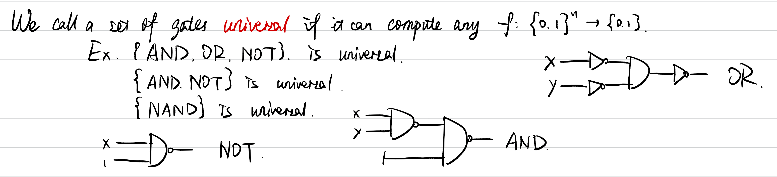
Before we break classical computing, we should be precise about what it can do. A set of gates is called universal if it can compute any function $f: \{0,1\}^n \rightarrow \{0,1\}$ .

Examples of universal sets include $\{\text{AND}, \text{OR}, \text{NOT}\}, \{\text{AND}, \text{NOT}\}$ , and the single gate $\{\text{NAND}\}$ .

1.2 The Need for Reversibility

Here is the catch. Standard classical gates like AND are not reversible because you cannot uniquely determine the inputs $$x, y$$ from the output $x \cdot y$ . Once you see the answer $$0$$ , you have no idea which of three inputs produced it. The information is simply gone. And that — the casual destruction of information — is exactly what quantum mechanics will not permit. In quantum computing, evolution must be reversible.

Why must it? It is not a design choice we are free to make; it is forced on us by the physics. Let us walk through the reasons one at a time, because each one is a clue to how quantum computers actually work.

The Unitary Nature of Quantum Mechanics: The time evolution of any closed quantum system is described by a Unitary Operator ($U$). In linear algebra, a matrix $U$ is unitary: $UU^\dagger = I$.
- Because $$U$$ has an inverse ( $U^\dagger$ ), you can always “undo” the operation.
- The evolution $$U$$ is derived from the Schrödinger Equation. When the Hamiltonian ( $$H$$ ) of a system is time-independent, the evolution is expressed as $e^{-iHt/\hbar}$ , which is inherently a unitary (and thus reversible) operator.
- Unitary transformations preserve the $$L_2$$ -norm (the total probability) of the quantum state, ensuring it remains exactly 1 throughout the evolution.
Information Conservation: In classical computing, operations like AND are irreversible because they discard information.
- No Information Loss: In a quantum system, information cannot be “deleted” or “lost” into thin air; it must be preserved within the system’s state.
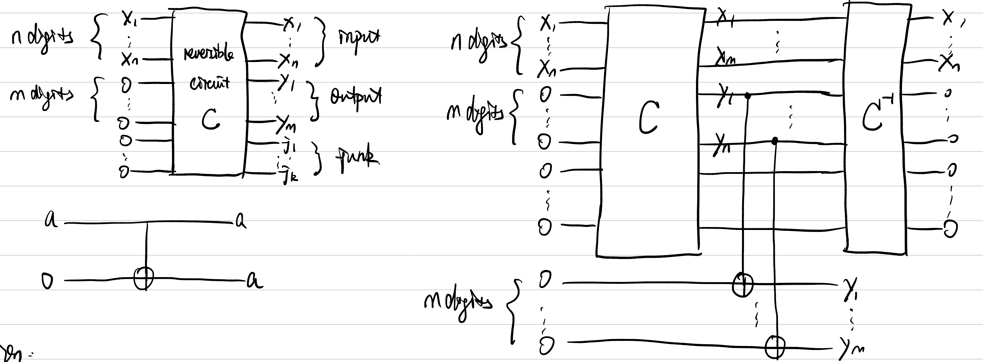
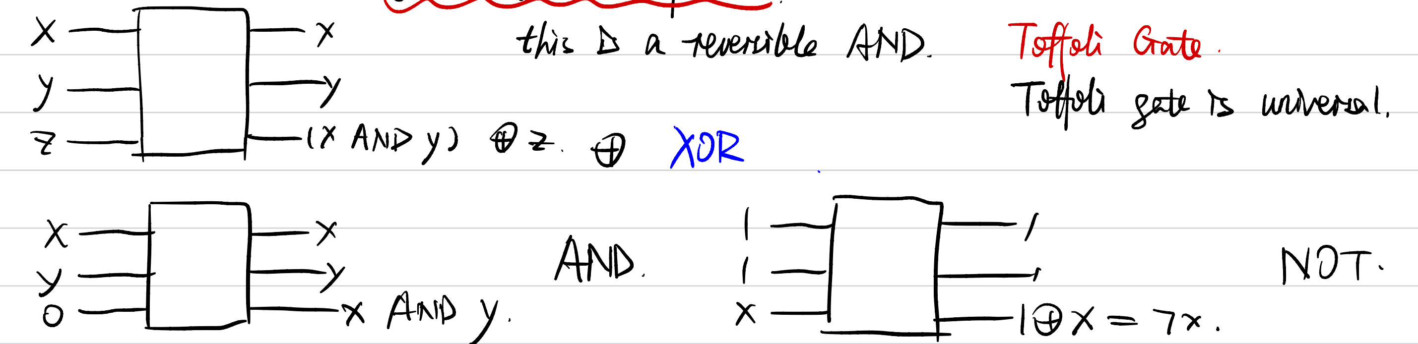
- The Toffoli Gate Example: To perform classical-style logic (like AND) in a quantum way, we use reversible gates like the Toffoli gate (Controlled-Controlled-NOT) which is also universal. This gate uses an Ancilla bit to store the result while keeping the original inputs intact, allowing the entire process to be reversed.
- Whenever we can compute $$f(x)$$ efficiently in polynomial time, we can efficiently compute the reversible mapping $(x, 0, 0) \mapsto (x, f(x), 0)$ .

The reassuring conclusion buried in that last bullet is worth saying plainly: insisting on reversibility costs us nothing in principle. Anything a classical computer can do efficiently, a reversible machine can do efficiently too — we just carry the inputs along instead of throwing them away.

Physical Heat and Landauer’s Principle: the physical reason for pursuing reversibility is often related to energy.
- Heat Generation: Landauer’s Principle states that erasing 1 bit of information releases a specific amount of heat into the environment.
- Energy Efficiency: Because quantum evolution is unitary (reversible), it theoretically does not require the erasure of information, which is a key requirement for building hardware that avoids the massive heat dissipation seen in classical high-performance chips.

So reversibility is not a quirk we tolerate — it is the very texture of quantum dynamics, and it even comes with a thermodynamic bonus. With that settled, we can finally ask what the thing being evolved actually is.

2. Postulates of Quantum Computing: States

2.1 The Qubit

A qubit is represented by a complex vector in a two-dimensional Hilbert space:

|\psi\rangle = \begin{pmatrix} \alpha \\ \beta \end{pmatrix} = \alpha|0\rangle + \beta|1\rangle

where $\alpha, \beta \in \mathbb{C}$ are amplitudes satisfying the normalization condition $|\alpha|^2 + |\beta|^2 = 1$ .

Read that normalization condition slowly, because it is doing real work. A classical bit sits at $$0$$ or $$1$$ , full stop. A qubit is allowed to be a weighted blend of both — but the weights are not free; their squared magnitudes must sum to one, so that “the probabilities add up.” That single constraint is the seed from which almost everything else grows.

Computational Basis: The vectors $|0\rangle = \binom{1}{0}$ and $|1\rangle = \binom{0}{1}$ form the standard basis for a qubit.
Dirac Notation:
- Ket $|\psi\rangle$ : A column vector.
- Bra $\langle \psi |$ : The conjugate transpose (dual vector) of a ket, represented as a row vector.
- Inner Product: $\langle \psi |\phi \rangle = a_0^* b_0 + a_1^* b_1$ .
- Outer Product: $|0\rangle\langle 0| + |1\rangle\langle 1|= I$ (the Identity matrix).

2.2 The Bloch Sphere

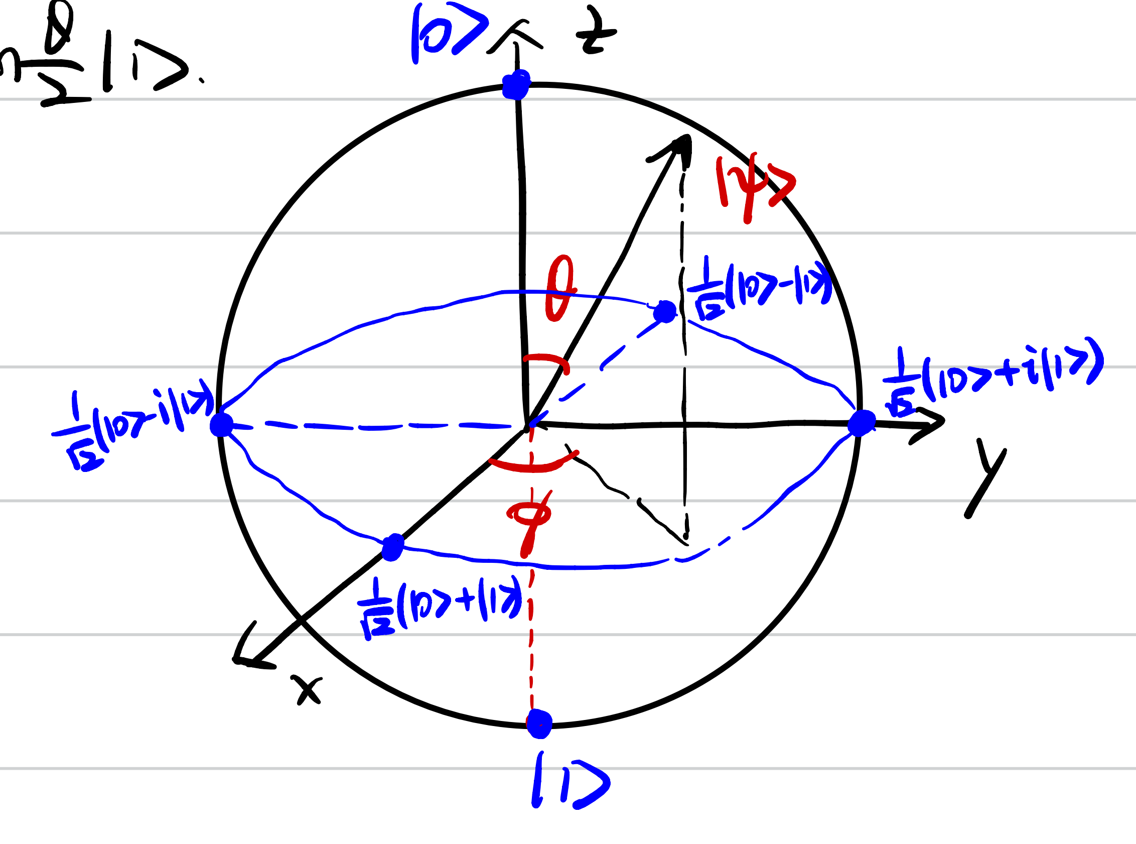
The algebra is fine, but two complex numbers tied down by one real constraint is hard to picture. Happily, there is a clean geometric home for a single qubit. Any single-qubit state can be visualized as a point on the Bloch Sphere using the following parameters:

|\psi\rangle = \cos\frac{\theta}{2}|0\rangle + e^{i\phi}\sin\frac{\theta}{2}|1\rangle

where $\theta$ and $\phi$ are real numbers defining the point’s coordinates. So the state of a qubit is, quite literally, a direction in space — a point on the surface of a sphere, with $|0\rangle$ at the north pole and $|1\rangle$ at the south. Every operation we apply to the qubit will turn out to be some rotation of this sphere, a picture we will lean on heavily in Part 2.

3. Quantum Dynamics

We have the state; now, how does it change? We already spoiled the answer back in Section 1, but let us state it as the postulate it is. The time evolution of a closed quantum system is described by a Unitary Transformation.

A matrix $$U$$ is unitary if $UU^\dagger = U^\dagger U = I$ .
This ensures that the state remains normalized: $\langle \psi | U^\dagger U | \psi \rangle = \langle \psi | \psi \rangle = 1$ .

That second line is the whole reason unitarity matters: it is precisely the condition that keeps “the probabilities adding up to one” true after the operation, not just before it. Now, which unitaries do we actually use in practice? A small handful show up again and again.

Common Single-Qubit Gates

Pauli Gates: $X = \begin{pmatrix} 0 & 1 \\ 1 & 0 \end{pmatrix}$ , $Y = \begin{pmatrix} 0 & -i \\ i & 0 \end{pmatrix}$ , $Z = \begin{pmatrix} 1 & 0 \\ 0 & -1 \end{pmatrix}$ .
Hadamard (H): $H = \frac{1}{\sqrt{2}}\begin{pmatrix} 1 & 1 \\ 1 & -1 \end{pmatrix}$ .
Phase Gates: $S = \begin{pmatrix} 1 & 0 \\ 0 & i \end{pmatrix}$ (Note: Corrected from notes) and $T = \begin{pmatrix} 1 & 0 \\ 0 & e^{i\pi/4} \end{pmatrix}$ .

Of these, the Hadamard deserves a special mention: hand it a crisp $|0\rangle$ and it returns an even blend of $|0\rangle$ and $|1\rangle$ . It is our standard tool for manufacturing superposition out of a definite state — and in a moment it will be the first move in building something far stranger.

4. Composite Systems and Entanglement

4.1 Tensor Products

One qubit is a sphere. What about two? You might guess we just keep a pair of spheres side by side — and for the simplest states, that is exactly right. The state space of a composite system is the tensor product of its individual component spaces. For example, if we have two qubits in states $|\psi\rangle$ and $|\phi\rangle$ , the combined state is $|\psi\rangle \otimes |\phi\rangle$ (often written as $|\psi\phi\rangle$ ).

4.2 Quantum Entanglement

But here is where the two-spheres intuition quietly breaks, and the real magic of quantum mechanics walks in.

Product States: States that can be written in the form $|\psi\rangle \otimes |\phi\rangle$ .
Entangled States: States that cannot be decomposed into a product of individual qubit states.
- Example: The state $\frac{1}{\sqrt{2}}(|00\rangle + |11\rangle)$ is entangled. Proof: Setting $\alpha_0\beta_1 = \alpha_1\beta_0 = 0$ while $\alpha_0\beta_0 = \alpha_1\beta_1 = \frac{1}{\sqrt{2}}$ leads to a contradiction.

Sit with that contradiction for a second, because it is not a technicality — it is the point. We tried to describe this two-qubit state as “qubit A is in some state, and separately qubit B is in some state,” and the algebra flatly refused. There is no such description. The pair has a joint reality that cannot be split into two private ones. Neither qubit has a state of its own; only the pair does. This is the resource that Part 2 will spend lavishly — on coding, on teleportation — and it is the cleanest signal that we have left the classical world for good.

Practical Implementation

Enough words. The Bell state $\frac{1}{\sqrt{2}}(|00\rangle + |11\rangle)$ we just called entangled is not an abstraction you have to take on faith — you can build it in a few lines and read the amplitudes straight off the screen. Notice the recipe is exactly the two moves we have been collecting: a Hadamard to make superposition, then a CNOT to bind the two qubits together.

from qiskit import QuantumCircuit
from qiskit.quantum_info import Statevector

# 1. Create a Bell State (Entangled State)
qc = QuantumCircuit(2)
qc.h(0)     # Apply Hadamard to the first qubit
qc.cx(0, 1) # Apply CNOT (controlled by q0, targeting q1)

# View the statevector
state = Statevector.from_instruction(qc)
print("Bell State Vector:")
print(state.data)

# 2. Apply a gate to a subsystem: (I ⊗ X) acting on the Bell state
qc.x(1) 
final_state = Statevector.from_instruction(qc)
print("\nState after (I ⊗ X):")
print(final_state.data)

So we have assembled the full toolkit: reversible (unitary) dynamics, the qubit and its Bloch sphere, the handful of gates that move it around, and the entanglement that two qubits can share. What we have studiously avoided is the one operation that actually pulls a classical answer out of all this quantum machinery — measurement. That turns out to be the subtlest piece of the whole story, and it is exactly where the interesting protocols live. That is where Part 2 begins. To be continued.